Interactive map
Explore province-level OOF R², A/B/C performance classes, and feature-importance layers in a single map.
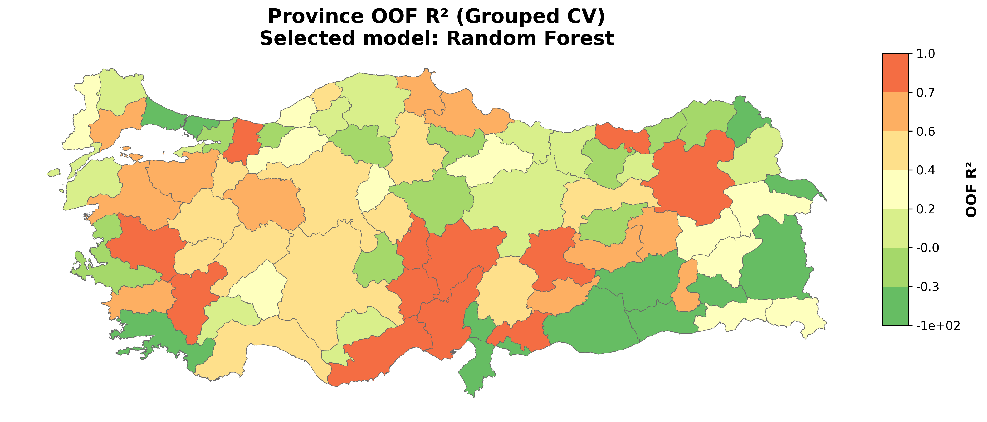
Province OOF R² (Grouped CV)
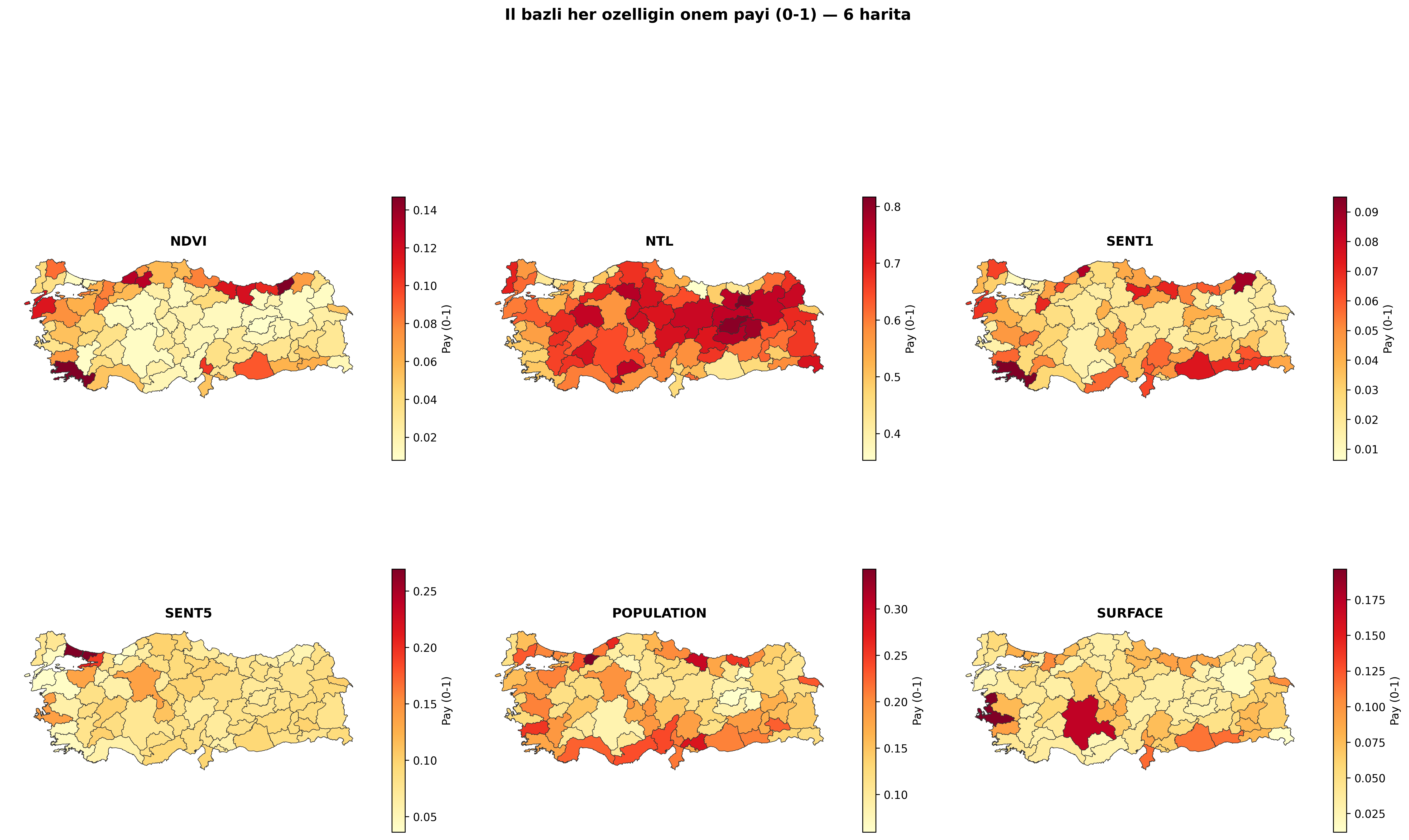
Province-level Out-of-Fold R² values. Selected model: Random Forest.
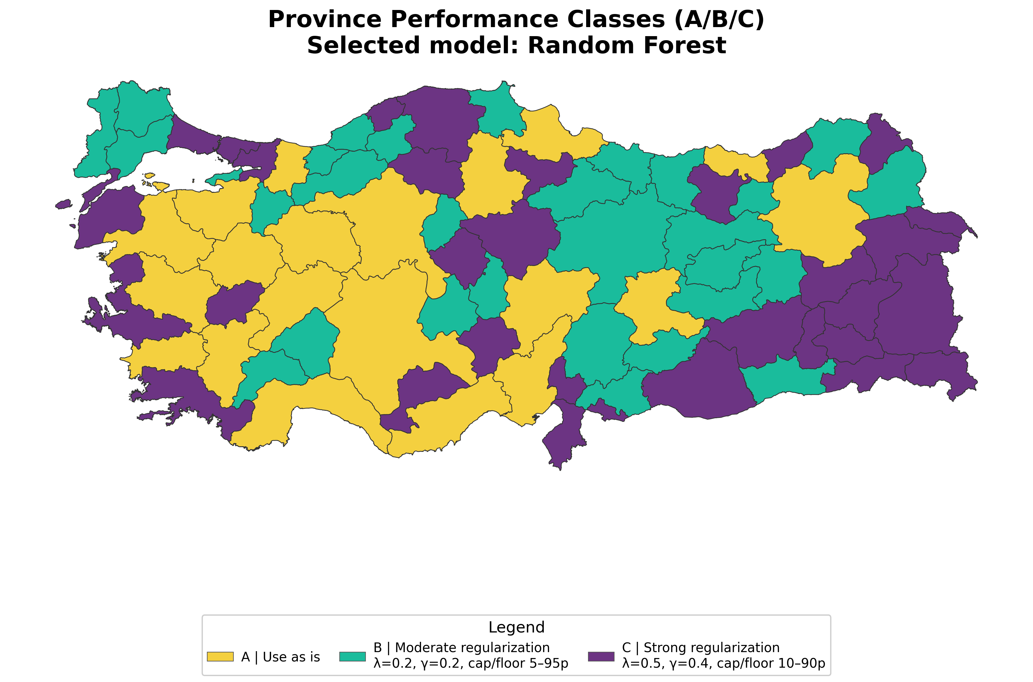
Province performance classes (A/B/C)
A: Use as is. B: Moderate regularization (λ=0.2, γ=0.2). C: Strong regularization (λ=0.5, γ=0.4).
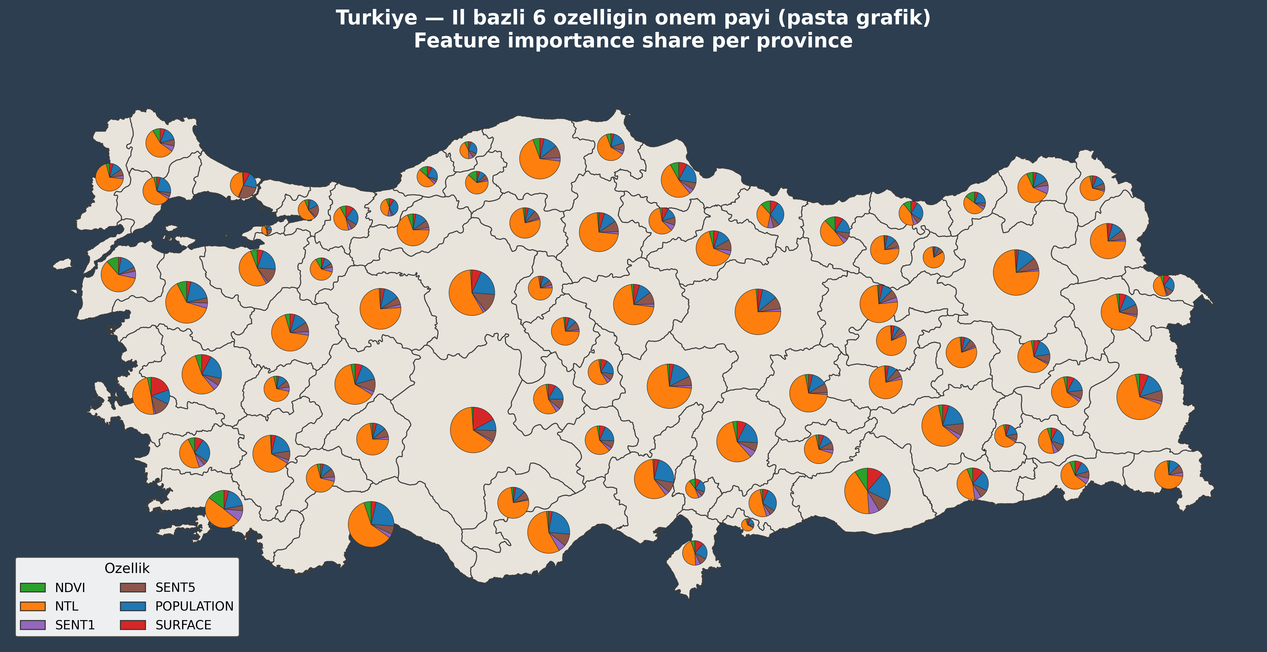
Feature-importance composition (province level)
Shares of NDVI, NTL, SENT1, SENT5, Population, and Surface. Use the embedded interactive chart and maps below to inspect values.
Interactive stacked bar chart
Six feature shares per province (stacked). Hover to see province name and percentages.
Interactive map — pie chart
Feature shares shown as a pie chart for each province. Click a province for details.
Static figures
Static versions of the same results.
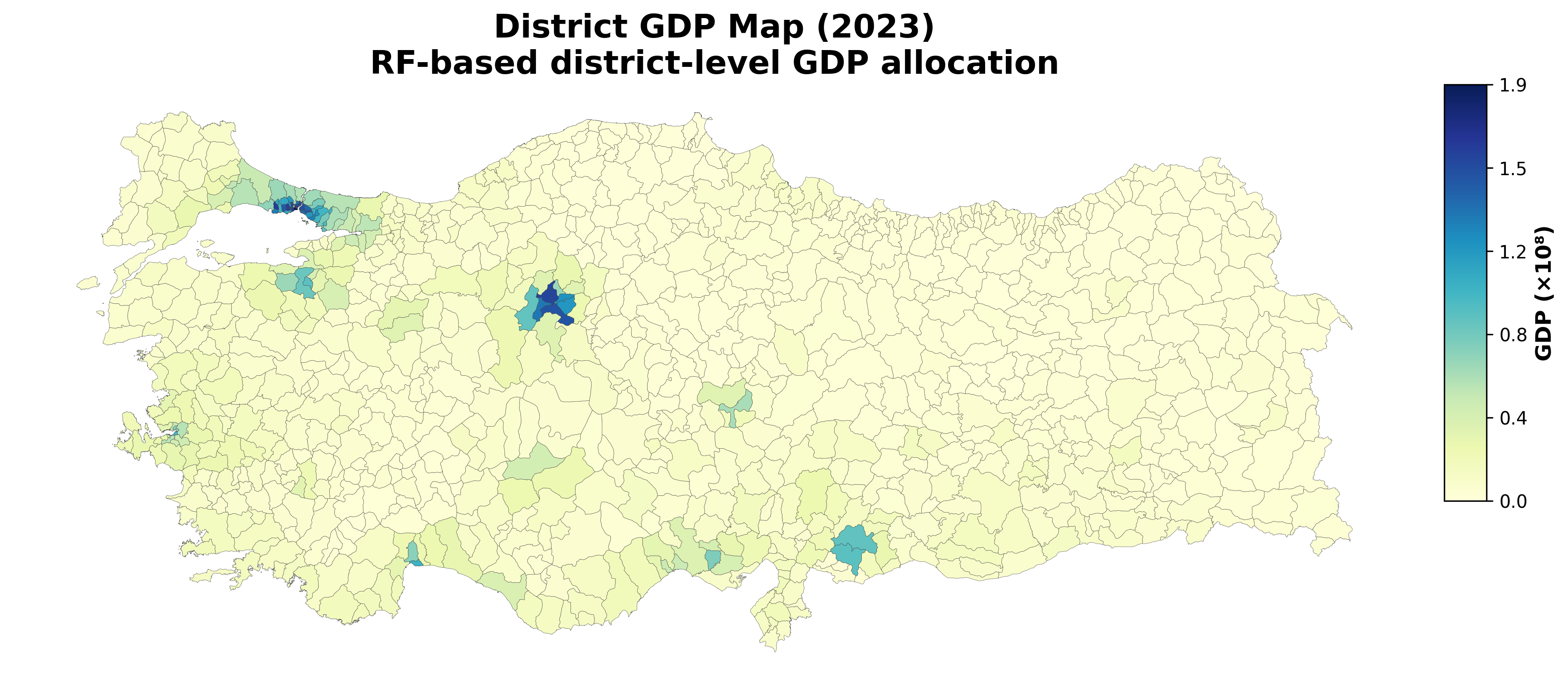
District GDP map (2023)
RF-based district-level GDP allocation. Use the province filter to focus on a single province or the full map; the color scale updates accordingly.
Tables
Numerical results for model comparison and robustness variants. Metric definitions and table intent are summarized below.
Table 1. Grouped cross-validation performance by model type
| Model | Type | N (provinces) | N (districts) | Features | CV R² | CV MSE | CV MAE | Selected |
|---|---|---|---|---|---|---|---|---|
| ElasticNet | Linear | 81 | 973 | 6 | 0.458 | 0.331 | 0.303 | — |
| SVR | Kernel | 81 | 973 | 6 | 0.448 | 0.337 | 0.285 | — |
| CatBoost | Boosting | 81 | 973 | 6 | 0.557 | 0.270 | 0.240 | — |
| RF | Bagging | 81 | 973 | 6 | 0.562 | 0.267 | 0.244 | Yes |
| XGBoost | Boosting | 81 | 973 | 6 | 0.516 | 0.295 | 0.259 | — |
| LightGBM | Boosting | 81 | 973 | 6 | 0.537 | 0.283 | 0.253 | — |
Purpose: Six model families are compared on the same dataset and feature set. Random Forest (RF) is selected with the highest CV R² (0.562) and the lowest CV MSE/MAE; subsequent district-level GDP allocation is reported using RF.
- RF slightly outperforms CatBoost and LightGBM in CV R², while linear models (ElasticNet, SVR) perform substantially worse.
- RF also achieves the best MSE and MAE, indicating lower prediction error.
- Grouped CV reduces leakage risk by keeping provinces separated across folds.
Table 2. Selected model summary (RF)
| N (provinces) | N (districts) | N (features) | CV R² | CV MSE | CV MAE |
|---|---|---|---|---|---|
| 81 | 973 | 6 | 0.562 | 0.267 | 0.244 |
Purpose: A one-row overview of the final setup used in the paper.
- R² ≈ 0.56 indicates moderate explanatory power at province-level grouped CV; remaining variance may reflect within-province structure and measurement uncertainty.
- MSE (0.267) and MAE (0.244) indicate acceptable error magnitudes given the target scale.
Table 3. Robustness variants — JS and L1 distance
| variant | JS_mean | JS_median | JS_max | L1_mean | n_province |
|---|---|---|---|---|---|
| GAM_minus | 2.61E-06 | 8.10E-07 | 3.99E-05 | 0.0027 | 81 |
| GAM_plus | 2.57E-06 | 8.72E-07 | 3.97E-05 | 0.0027 | 81 |
| LAM_minus | 2.02E-06 | 7.67E-07 | 2.10E-05 | 0.0025 | 81 |
| LAM_plus | 1.96E-06 | 8.40E-07 | 2.22E-05 | 0.0025 | 81 |
| THR_Aminus | 9.37E-06 | 0 | 3.32E-04 | 0.0015 | 81 |
| THR_Aplus | 1.62E-05 | 0 | 1.15E-03 | 0.0016 | 81 |
| THR_Bminus | 3.54E-08 | 0 | 2.87E-06 | 0.0000 | 81 |
| THR_Bplus | 2.04E-06 | 0 | 1.45E-04 | 0.0005 | 81 |
Purpose: Quantify how feature-importance shares change under gamma/lambda (GAM/LAM) and threshold (THR) perturbations. THR_Bminus is the most stable variant with minimal JS and L1.
- THR_Bminus is closest to the reference (JS_mean ≈ 3.5e-08; L1_mean = 0).
- THR_Aplus yields the largest deviation (JS_max 1.15e-03), indicating A-class threshold changes shift feature importance more.
- GAM/LAM variants remain close to each other, suggesting stability within a reasonable parameter range.
GDP vs. SES and RWI (2023)
Relationship between district GDP and socioeconomic score (SES) / relative wealth index (RWI).
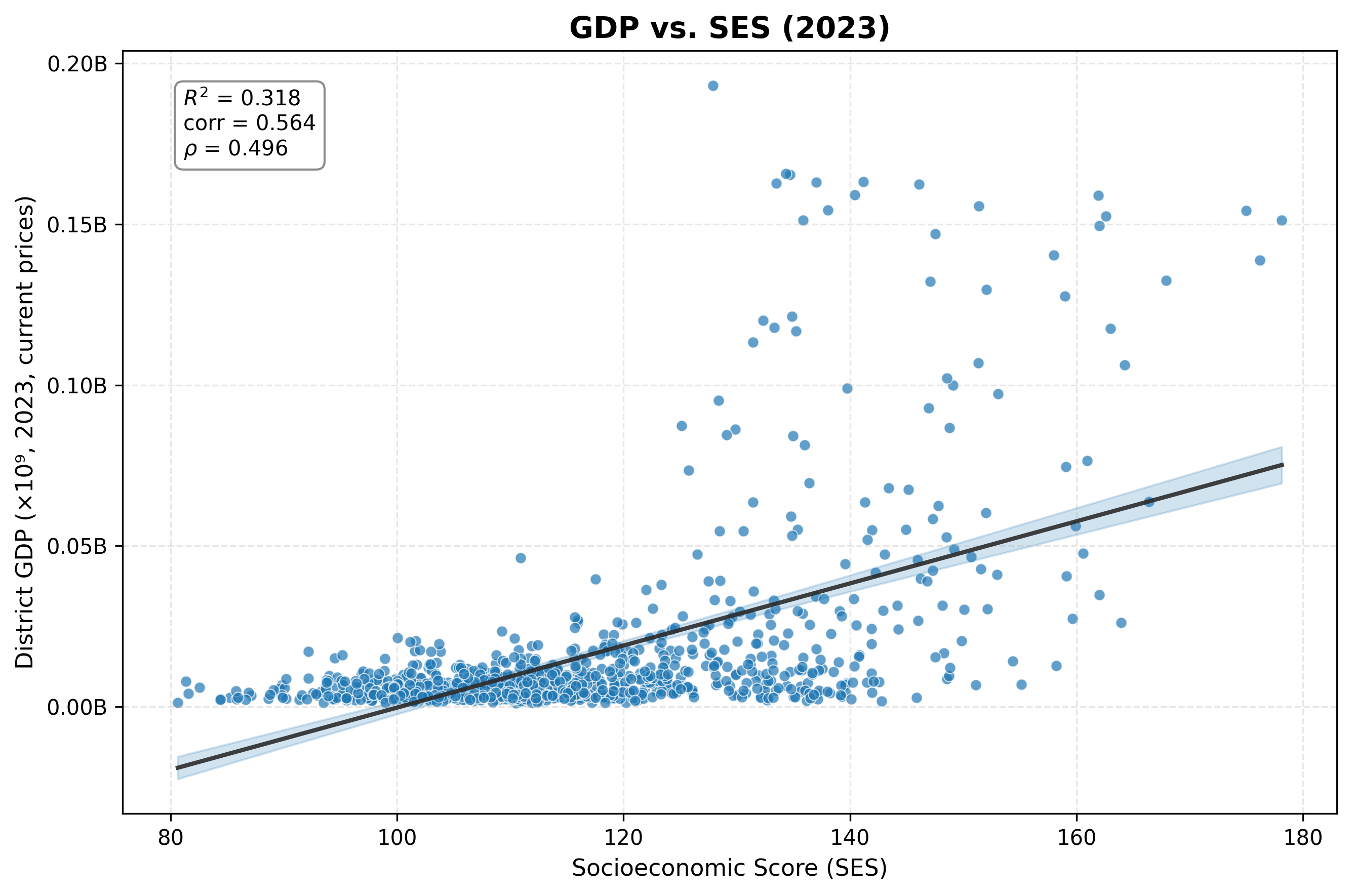
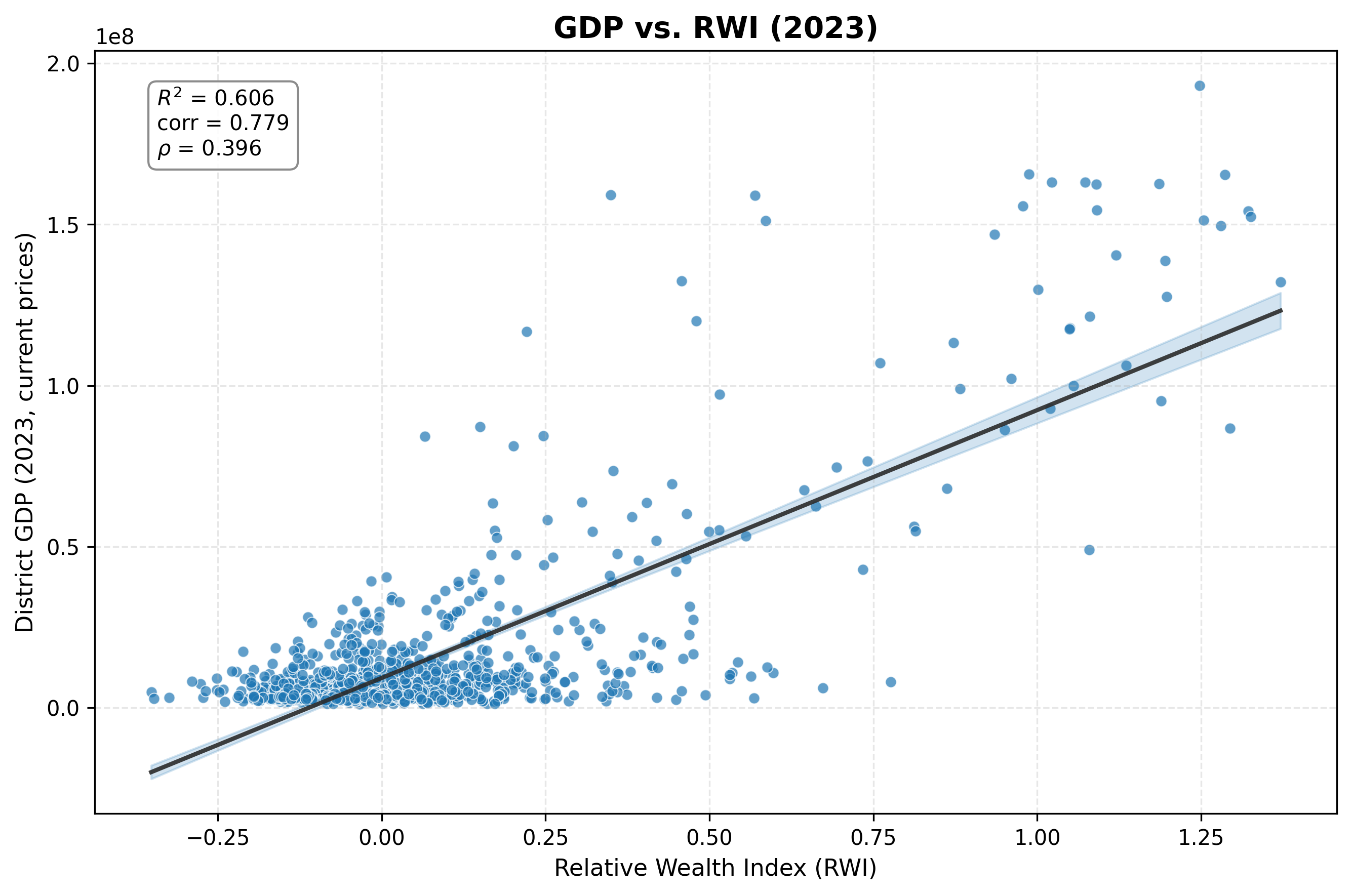
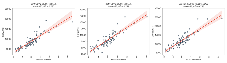
Empirical validation of SEDI’s core assumption (NUTS-3)
Purpose: test whether the SEDI distribution mirrors macroeconomic reality using official GDP per capita (development density), rather than total GDP (population-confounded).